Reinforcement Learning Lesson 1

This is the first post for the series reinforcement learning. The main source for the entire series is here. The post mainly focus on summarizing the content introduced in the video and slides, as well as some of my own understanding. Any feedback is welcomed.

In this post, we will talk about Markov Decision Process (MDP), which is a pretty fundamental model in many reinforcement learning cases.

Almost all RL problems can be formalized as MDP

Markov Process

In order to learn about MDP, we need to first know what is Markov Process (MP). This introduces the following two concept:

• Markov Property
• State Transition Matrix

In the most simple word, Markov Property means that the future state is independent on the history given the current state. It can be formalized using following statement:

\[\mathbb{P}[S_{t+1}|S_{t}] = \mathbb{P}[S_{t+1}|S_1, ..., S_t]\]

This means that the current state contains all they necessary information for the future, and we can discard all history information.

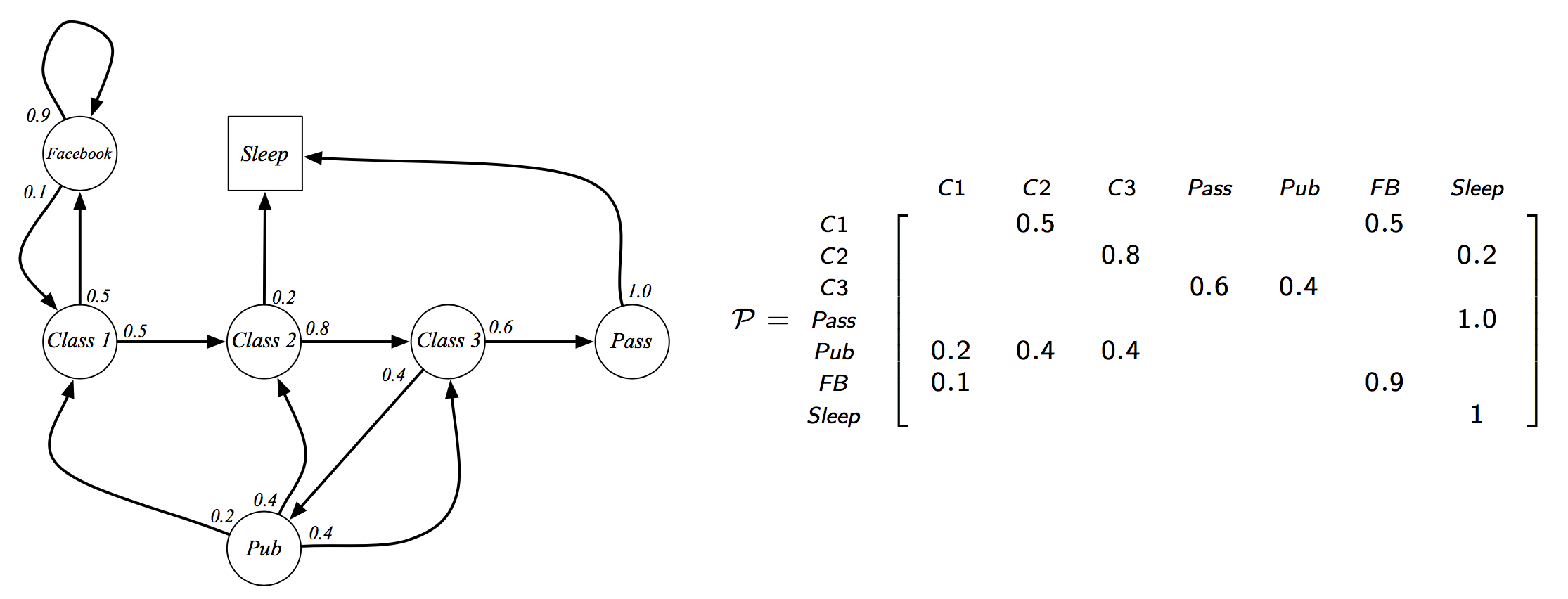
State Transition Matrix contains the probability we go from on state to another one. Given a state \( s \) and its successor state \( s^\prime \), the probability from \( s \) goes to \( s^\prime \) is given by

\[P_{ss\prime} = \mathbb{P}[S_{t+1}=s\prime|S_{t}=s]\]

And the State Transition Matrix is by

\[P = \begin{Bmatrix} P_{11} & ... & P_{1n} \\ \vdots & ... & \vdots \\ P_{n1} & ... & P_{nn} \end{Bmatrix}\]

From the above two concept, we can notice two things and these are also the constraint for MDP:

• The state is finite (otherwise the definition of State Transition Matrix is problematic)
• The environment is fully observable, no hidden state exists

We can obtain a definition for MP as a tuple \( <S, P> \):

• \( S \) is a finite state set
• \( P \) is a state transition matrix

An example of MP:

Markov Reward Process

Markov Process combined with values, then we have Markov Reward Process (MRP), defined by a tuple \( <S, P, R, \gamma> \):

• \( S \) is a finite state set
• \( P \) is a state transition matrix
• \( R \) is a reward function, \(R_{s} = \mathbb{E}[R_{t+1}|S_{t}=s]\)
• \( \gamma \) is a discounting ratio

As we have introduced reward, we can measure how many rewards we can get in each state. We define return \( G_t \) as the discounted rewards we can get from timestamp \( t \), and state value function \( v(s) \) the expected return we can get starting from state \( s \):

\[G_t = R_{t+1} + \gamma R_{t+2} + ... = \sum_{k=1}^{\infty}\gamma^{k}R_{t+k+1}\] \[v(s) = \mathbb{E}[G_t|S_t=s]\]

Note that the return is accumulated with discounting. This is important is:

• Avoid infinity loop that might exist in MDP (e.g. self loop)
• Model the uncertainty about the future
• From common sense, human prefer immediate reward than long term ones

We can breakdown the state value function into two parts, immediate and long term. Using recurse, we have the Bellman Equation for MRP:

\[v(s) = \mathbb{E}[R_{t+1} + \gamma v(S_{t+1})|S_t=s]\]

By expanding the above expectation and using sum to replace expectation operator, we have:

\[v(s) = R_s + \gamma\sum_{s^\prime\in S}P_{ss^\prime}v(s^\prime)\]

Markov Decision Process

Adding the actions we can make among the state, we finally have the definition for MDP, which is \( <S, A, P, R, \gamma> \):

• \( S \) is a finite state set
• \( A \) is a finite action set
• \( P \) is a state transition matrix, \(P_{ss^\prime}^a = \mathbb{P}[S_{t+1}=s^\prime|S_{t}=s, A_t=a]\)
• \( R \) is a reward function, \(R_{s}^a = \mathbb{E}[R_{t+1}|S_{t}=s, A_t=a]\)
• \( \gamma\) is a discounting ratio

Notice the change on the state transition matrix, before we only have a single matrix, and now we have one for each action \( a \) we can think of in the pervious case, we have only single action). Under different action \( a \), the transition probability can be different between the two state. We can now regard the new state transition matrix as a tensor with three dimension.

As we have actions to now, we need to make decision how to take actions. A policy is a distribution over actions given a state:

\[\pi(a|s) = \mathbb{P}[A_t=a|S_t=s]\]

A policy fully determines how an agent would act, and it does not depend on the history. Similar to MRP, we have state value function for MDP as the expected return starting from \( s \), following the policy \( \pi \):

\[v_{\pi}(s) = \mathbb{E}_{\pi}[G_t|S_t=s]\]

We can also define an action value function, which is the expected return we get starting from state \( s \), taking action \( a \) and following policy \( \pi \):

\[q_{\pi}(s, a) = \mathbb{E}_{\pi}[G_t|S_t=s, A_t=a]\]

These two functions have relationship and can be transformed to each other easily, to get state value function, we can summation over all the action value function for the action that state we could get, weight by the policy:

\[v_\pi(s) = \sum_{a\in A}\pi(a|s)q_{\pi}(s, a)\]

And the action value function can be obtained by summation overall all state we can transition to, weighted by the state transition matrix:

\[q_\pi(s, a) = R_s^a + \gamma\sum_{s^\prime}P_{ss^\prime}^a v(s^\prime)\]

Combine the above equations, we can obtain the Bellman Exception Equation as:

\[v_\pi(s) = \sum_{a\in A}\pi(a|s)(R_s^a + \gamma\sum_{s^\prime}P_{ss^\prime}^a v(s^\prime))\] \[q_\pi(s, a) = R_s^a + \gamma\sum_{s^\prime}P_{ss^\prime}^a \sum_{a\in A}\pi(a|s^\prime)q_{\pi}(s^\prime, a)\]

Given a MDP, if we want to solve it (to know what’s the best performance we can get, e.g. What’s the maximum rewards we can get in the terminate state), we need to find the optimal value function for it. As long as we have obtain the optimal value function, we can compose an optimal policy easily:

\[\pi_{*}(a|s) = \begin{cases} 1, & \text{if $a = argmax_{a\in A} q(s, a)$} \\ 0, & \text{otherwise} \end{cases}\]

There exists an optimal policy \( \pi_{*} \) that is better than or equal to all other policy for any MDP. All optimal policy achieve optimal state value function and optimal action value function

Following this policy, we can change our Bellman Exception Equation to Bellman Optimality Equation:

\[v_*(s)=max_{a}(R_s^a + \gamma\sum_{s^\prime\in S}P_{ss^\prime}^a v_*(s^\prime))\] \[q_*(s, a)=R_s^a + \gamma\sum_{s^\prime\in S} argmax_{a} P_{ss^\prime}^a v_*(s^\prime)\]

Bellman Optimality Equation is non-linear, there is no closed form solution for it. However, we can solve it by some iterative methods (will introduce in later lectures):

• Policy Iteration
• Value Iteration
• Q-learning
• Sarsa