A Random Walk Down Recsys - Part 4

Welcome back to the fourth installment of A Random Walk Down Recsys. This time, the three papers span a range of practical challenges in generative recommendation: efficiently compressing long user sequences through recurrent memory, accelerating constrained decoding on hardware accelerators via trie vectorization, and rethinking how semantic IDs are trained and maintained with a dynamic, end-to-end item tokenizer. Together, they represent advances on three different fronts — training efficiency, serving performance, and SID lifecycle management.

The three papers covered are: Recurrent Preference Memory (Tencent), Vectorizing the Trie (Google), and PIT (Kuaishou).

Recurrent Preference Memory: Compressing Long Sequences via Learnable Tokens

This Tencent paper addresses a central challenge in generative recommendation: how to efficiently compress long user behavior sequences while supporting incremental updates for both space and time optimization.

Core Idea: Segmented Sequence Compression

The key insight is to partition user sequences into segments and compress each segment through a learnable memory token. At prediction time, the model only needs to consume these memorized tokens rather than the full history — dramatically reducing the input length.

This idea shares conceptual DNA with Meta’s earlier work on Efficient Sequential Recommendation for Long Term User Interest Via Personalization, which also uses learnable tokens to compress sequence segments. Both approaches employ a “decoder as encoder” strategy, applying causal masking within each segment so that information flows forward naturally.

Training Approaches and Their Trade-offs

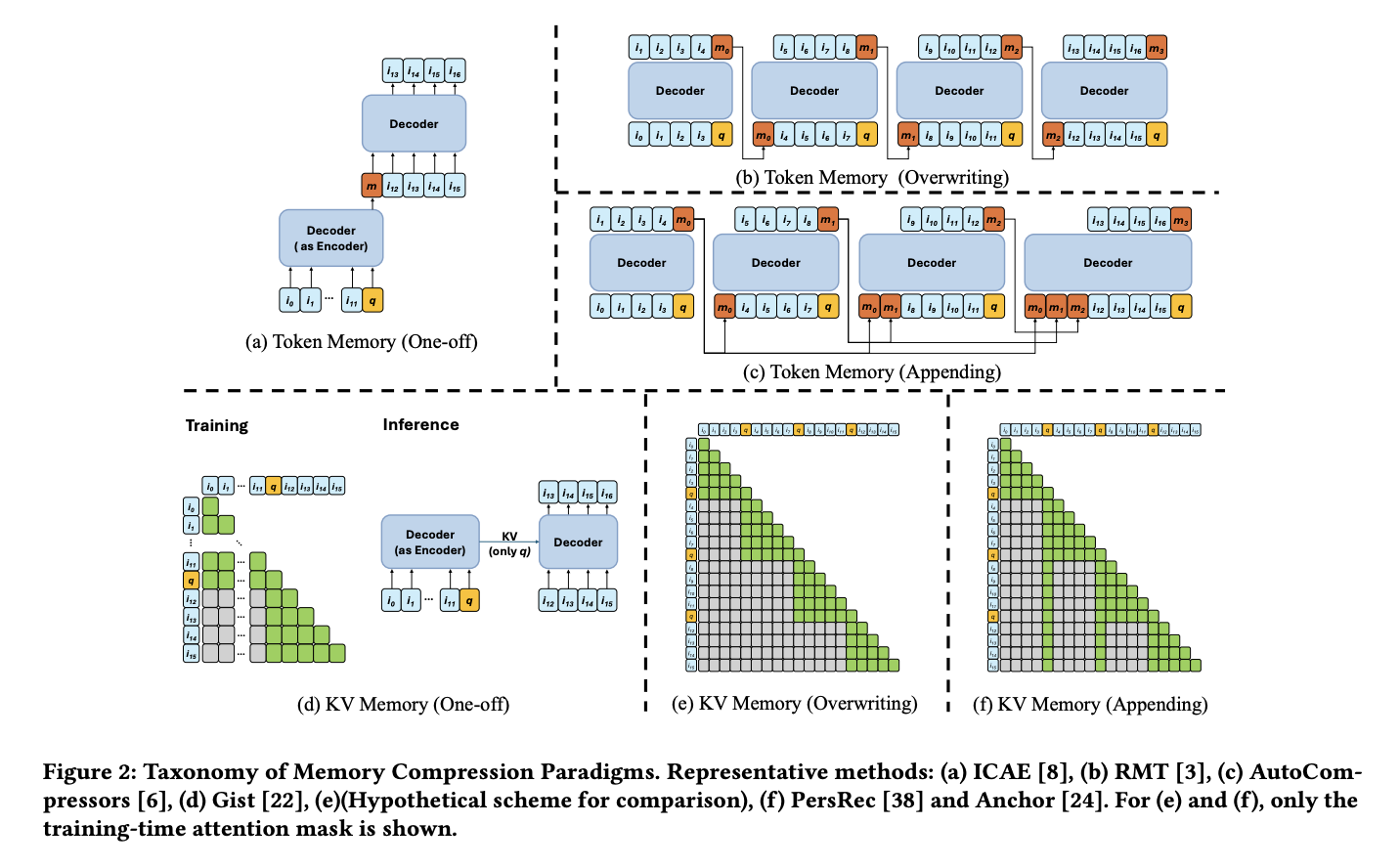
The paper surveys several training strategies for the recurrent memory update:

• Recurrent update (approaches b and c in the paper): A straightforward RNN-style sequential update. Each segment’s memory depends on the previous segment’s output, introducing long latency due to the inherently sequential nature of the computation.
• Masked parallel (approaches e and f): Uses attention masking to enable parallel processing across segments. However, this requires storing the KV cache for every layer, leading to significant memory overhead. (Though it is worth noting that during incremental updates, these approaches should not need to retain all historical KV caches — this point could use further clarification.)

Self-Reflection Teacher Forcing

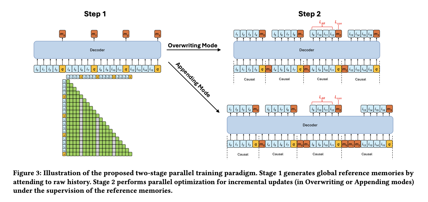
To resolve the tension between sequential dependency and parallel efficiency, the authors propose self-reflection teacher forcing, a two-stage training procedure:

Stage 1 — Global Reference Memory Generation: A memory token is inserted into each segment. All items within a segment can attend to preceding items via standard causal attention, but critically, they cannot attend to the memory token. This produces a “global reference memory” — an uncontaminated summary of each segment.

Stage 2 — Sub-Sequence Parallel Training: Each sub-sequence is processed in parallel. Within each segment, items attend to:

• The global reference memory tokens from all preceding segments
• The current segment’s items and its memory token

The updated memory token is then trained to match the global reference memory via an MSE loss — this is the “teacher” component. The reference memory acts as a supervision signal, guiding the incrementally updated memory to converge toward the same representation that a full-context model would produce.

This design elegantly enables masked parallelism during training while ensuring that the recurrent memory tokens learn to faithfully compress segment information.

Vectorizing the Trie: Accelerator-Friendly Constrained Decoding for SID Beam Search

This Google paper tackles a performance-critical problem in generative retrieval: how to vectorize a trie (prefix tree) for efficient constrained beam search on hardware accelerators like TPUs and GPUs.

High-Level Approach

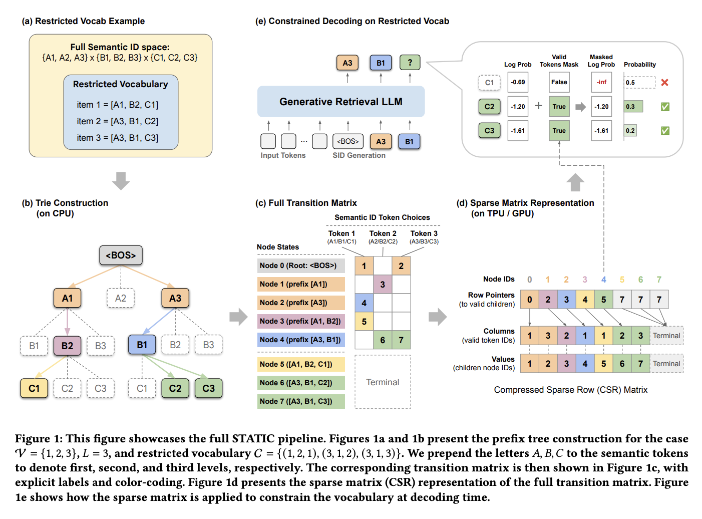
The approach differs from typical trie implementations in a key way: every prefix in the trie is assigned a unique node ID, and a transition matrix records which nodes can be reached from any given node. This transforms the tree traversal problem into a series of matrix lookups that are naturally suited to accelerator hardware.

The index building process uses a two-tier strategy:

• Top layers: A dense multi-dimensional tensor provides O(1) direct indexing for the initial decoding steps, where the branching factor is manageable and fast lookup is critical.
• Deeper layers: A Compressed Sparse Row (CSR) representation handles the sparser, deeper portions of the trie, where a dense tensor would waste too much memory.

The detail code could be viewed here: static-constraint-decoding. The following section provides a detailed walkthrough of the build_static_index function with some toy examples to better illustrate the idea.

Deep Dive: build_static_index

This walkthrough covers the build_static_index function in static_decoding/csr_utils.py. The function converts a sorted array of Semantic IDs into a static, accelerator-friendly trie representation using the hybrid dense/CSR approach described above.

Throughout this guide we use the following running example:

fresh_sids = np.array([
    [1, 3, 5, 7],   # row 0
    [1, 3, 5, 9],   # row 1
    [1, 3, 6, 2],   # row 2
    [1, 4, 2, 1],   # row 3
    [2, 1, 1, 1],   # row 4
])
vocab_size = 10
dense_lookup_layers = 2
# N=5 sequences, each of length L=4

This corresponds to a trie that looks like:

             root
            /    \
          1       2
         / \       \
        3   4       1
       / \   \       \
      5   6   2       1
     / \   \   \       \
    7   9   2   1       1

---

Section 1: Initial Level-0 Mask

start_mask = np.zeros(vocab_size, dtype=bool)
start_mask[np.unique(fresh_sids[:, 0])] = True

What it does: Creates a boolean vector of length vocab_size indicating which tokens are valid at the very first position (the root’s children).

Running example: fresh_sids[:, 0] is [1, 1, 1, 1, 2], so np.unique(...) = [1, 2].

start_mask = [F, T, T, F, F, F, F, F, F, F]
              0  1  2  3  4  5  6  7  8  9

Only tokens 1 and 2 are valid starting points.

---

Section 2: Vectorized Trie Node Identification

Step 2a: Consecutive row differences

diff = (fresh_sids[1:] != fresh_sids[:-1])

Compares each consecutive pair of rows element-wise, producing a boolean matrix of shape (N-1, L):

row 0 vs 1: [1≠1, 3≠3, 5≠5, 7≠9] → [F, F, F, T]
row 1 vs 2: [1≠1, 3≠3, 5≠6, 9≠2] → [F, F, T, T]
row 2 vs 3: [1≠1, 3≠4, 6≠2, 2≠1] → [F, T, T, T]
row 3 vs 4: [1≠2, 4≠1, 2≠1, 1≠1] → [T, T, T, F]

Step 2b: Find the shallowest divergence depth

first_diff = np.full(N - 1, L, dtype=np.int8)
has_diff = diff.any(axis=1)
first_diff[has_diff] = diff[has_diff].argmax(axis=1)

• first_diff is initialized to L (sentinel for “no difference”).
• has_diff flags which row pairs differ at all.
• argmax on a boolean row returns the index of the first True — the shallowest depth where the two sequences diverge.

first_diff = [3, 2, 1, 0]

Interpretation:

• Rows 0→1 first differ at depth 3 (share prefix [1,3,5])
• Rows 1→2 first differ at depth 2 (share prefix [1,3])
• Rows 2→3 first differ at depth 1 (share prefix [1])
• Rows 3→4 first differ at depth 0 (completely different roots)

Step 2c: Build the is_new matrix

is_new = np.zeros((N, L), dtype=bool)
is_new[0, :] = True
for depth in range(L):
    is_new[1:, depth] = (first_diff <= depth)

A trie node at (row, depth) is “new” if the sequences diverged at or before that depth. The first row is always entirely new.

is_new = [[T, T, T, T],   # row 0: first row, all new
          [F, F, F, T],   # row 1: same prefix [1,3,5], only leaf is new
          [F, F, T, T],   # row 2: same [1,3], new from depth 2 onward
          [F, T, T, T],   # row 3: same [1], new from depth 1 onward
          [T, T, T, T]]   # row 4: entirely new root, all new

---

Section 3: State ID Assignment

Every unique trie node (prefix) is assigned a unique integer State ID.

Depth 0: Token-based IDs

state_ids = np.zeros((N, L - 1), dtype=np.int32)
state_ids[:, 0] = fresh_sids[:, 0].astype(np.int32) + 1

Level-0 IDs are simply token_value + 1, reserving 0 as a null state. These IDs occupy the range [1, vocab_size].

state_ids[:, 0] = [2, 2, 2, 2, 3]

Deeper depths: Sequential ID assignment with maximum.accumulate

depth_id_ranges = []
current_offset = vocab_size + 1  # = 11

for depth in range(1, L - 1):
    mask = is_new[:, depth]
    num_new = np.sum(mask)
    start_id = current_offset
    end_id = current_offset + num_new

    depth_id_ranges.append((start_id, end_id))

    state_ids[mask, depth] = np.arange(start_id, end_id, dtype=np.int32)
    state_ids[:, depth] = np.maximum.accumulate(state_ids[:, depth])
    current_offset += num_new

For each depth beyond 0:

1. mask: which rows introduce a new trie node at this depth.
2. Assign IDs: consecutive integers starting from current_offset, placed only at “new node” rows.
3. maximum.accumulate: since the data is sorted, rows sharing the same prefix are contiguous. After placing IDs at boundary rows, the gaps (zeros) are filled forward by propagating the most recent non-zero ID.

Depth 1 — is_new[:, 1] = [T, F, F, T, T], 3 new nodes → IDs 11, 12, 13:

Before accumulate: [11,  0,  0, 12, 13]
After accumulate:  [11, 11, 11, 12, 13]

Depth 2 — is_new[:, 2] = [T, F, T, T, T], 4 new nodes → IDs 14, 15, 16, 17:

Before accumulate: [14,  0, 15, 16, 17]
After accumulate:  [14, 14, 15, 16, 17]

Final state_ids matrix:

        depth 0   depth 1   depth 2
row 0: [  2,       11,       14  ]   ← path for [1, 3, 5, 7]
row 1: [  2,       11,       14  ]   ← path for [1, 3, 5, 9]
row 2: [  2,       11,       15  ]   ← path for [1, 3, 6, 2]
row 3: [  2,       12,       16  ]   ← path for [1, 4, 2, 1]
row 4: [  3,       13,       17  ]   ← path for [2, 1, 1, 1]

Total states: num_states = 18 (0 is null, 1–10 are level-0, 11–17 are deeper).

---

Section 4: Edge Collection

all_parents, all_tokens, all_children = [], [], []
for depth in range(1, L):
    mask = is_new[:, depth]
    parent_ids = state_ids[mask, depth-1]
    token_ids = fresh_sids[mask, depth].astype(np.int32)
    child_ids = (
        state_ids[mask, depth] if depth < L - 1
        else np.zeros_like(parent_ids, dtype=np.int32)
    )
    all_parents.append(parent_ids)
    all_tokens.append(token_ids)
    all_children.append(child_ids)

For each new trie node, an edge is (parent_state, token) → child_state. At the last depth (depth == L-1), nodes are leaves so the child state is 0 (terminal).

Running example edges:

Parent State	Token	Child State	Prefix represented
2	3	11	[1] → token 3 → [1,3]
2	4	12	[1] → token 4 → [1,4]
3	1	13	[2] → token 1 → [2,1]
11	5	14	[1,3] → token 5 → [1,3,5]
11	6	15	[1,3] → token 6 → [1,3,6]
12	2	16	[1,4] → token 2 → [1,4,2]
13	1	17	[2,1] → token 1 → [2,1,1]
14	7	0	[1,3,5] → token 7 (leaf)
14	9	0	[1,3,5] → token 9 (leaf)
15	2	0	[1,3,6] → token 2 (leaf)
16	1	0	[1,4,2] → token 1 (leaf)
17	1	0	[2,1,1] → token 1 (leaf)

---

Section 5: Dense Specialization

dense_shape = tuple([vocab_size] * dense_lookup_layers)
dense_mask = np.zeros(dense_shape, dtype=bool)
dense_states = np.zeros(dense_shape, dtype=np.int32)

indices = tuple(
    fresh_sids[:, i].astype(np.int32) for i in range(dense_lookup_layers)
)
final_dense_ids = state_ids[:, dense_lookup_layers - 1]

dense_mask[indices] = True
dense_states[indices] = final_dense_ids

For the first dense_lookup_layers depths, a dense multi-dimensional tensor provides O(1) direct indexing — much faster than sparse lookups for the “hot” initial decoding steps.

With dense_lookup_layers=2, both tensors are (10, 10):

• dense_mask[t0, t1]: Is the prefix [t0, t1] valid?
• dense_states[t0, t1]: What state ID does prefix [t0, t1] lead to?

The index tuple (fresh_sids[:, 0], fresh_sids[:, 1]) = ([1,1,1,1,2], [3,3,3,4,1]) addresses exactly the cells for existing prefixes.

Result (non-zero entries only):

Cell	dense_mask	dense_states	Meaning
[1, 3]	True	11	Prefix [1, 3] → state 11
[1, 4]	True	12	Prefix [1, 4] → state 12
[2, 1]	True	13	Prefix [2, 1] → state 13
all others	False	0	Invalid prefix

Rows 0–2 all write to [1, 3] with the same state ID 11 — safe because they share the same prefix.

---

Section 6: CSR Construction

parents = np.concatenate(all_parents)
tokens = np.concatenate(all_tokens)
children = np.concatenate(all_children)

counts = np.bincount(parents, minlength=num_states)
indptr = np.zeros(num_states + 1, dtype=np.int32)
indptr[1:] = np.cumsum(counts)

The edges from Section 4 are flattened into parallel arrays. Then a standard CSR indptr is built:

• counts[s] = number of outgoing edges from state s.
• indptr[s] to indptr[s+1] gives the slice of tokens/children belonging to state s.

To look up valid transitions from state s:

valid_tokens = tokens[indptr[s]:indptr[s+1]]
next_states  = children[indptr[s]:indptr[s+1]]

---

Section 7: Layer Max Branches

layer_max_branches = [np.sum(start_mask)]

l0_counts = counts[1:vocab_size + 1]
layer_max_branches.append(int(l0_counts.max()) if len(l0_counts) > 0 else 0)

for (start_id, end_id) in depth_id_ranges:
    if start_id < len(counts):
        layer_counts = counts[start_id:end_id]
        layer_max_branches.append(
            int(layer_counts.max()) if len(layer_counts) > 0 else 0
        )
    else:
        layer_max_branches.append(0)

while len(layer_max_branches) < L:
    layer_max_branches.append(1)

Accelerator compilers (XLA, TorchScript) require static tensor shapes. This section computes the worst-case (maximum) number of child tokens any single node can have at each trie depth:

Depth	Source	Nodes examined	Max children
0	Root	root	2 (tokens 1, 2)
1	Level-0 states (IDs 1–10)	states for tokens 1, 2	2 (token 1 → children 3, 4)
2	Depth-1 states (IDs 11–13)	states 11, 12, 13	2 (state 11 → children 5, 6)
3	Depth-2 states (IDs 14–17)	states 14, 15, 16, 17	2 (state 14 → children 7, 9)

Result: layer_max_branches = (2, 2, 2, 2).

The compiler uses these values to allocate fixed-size buffers at each decoding step.

---

Section 8: Final Packing

raw_indices = np.concatenate(
    [tokens, np.full(vocab_size, vocab_size, dtype=np.int32)]
)
raw_data = np.concatenate([children, np.zeros(vocab_size, dtype=np.int32)])
indptr = np.append(indptr, indptr[-1] + vocab_size)

packed_csr = np.ascontiguousarray(np.vstack([raw_indices, raw_data]).T)

Padding state

A dummy “padding state” with vocab_size fake entries is appended:

• Token values are set to vocab_size (out-of-vocabulary — will never match a real token).
• Child states are set to 0 (the null state).
• indptr is extended by one entry so the padding state’s edges are properly bounded.

This ensures that if a compiled kernel ever indexes an invalid or terminal state, it reads harmless dummy data instead of causing an out-of-bounds access — enabling branchless, hardware-friendly execution.

Packed CSR format

tokens and children are interleaved into a 2D array of shape (num_edges + vocab_size, 2):

packed_csr = [[token_0, child_0],
              [token_1, child_1],
              ...
              [vocab_size, 0],   ← padding
              [vocab_size, 0],   ← padding
              ...]

np.ascontiguousarray ensures the memory layout is sequential in C order for optimal GPU HBM burst throughput.

Return values

return packed_csr, indptr, tuple(layer_max_branches), start_mask, dense_mask, dense_states

Return value	Shape	Purpose
packed_csr	(num_edges + V, 2)	Flat [token, next_state] transition table
indptr	(num_states + 2,)	CSR row pointers into packed_csr
layer_max_branches	(L,)	Max branching factor per depth (for static shapes)
start_mask	(V,)	Valid first-token mask
dense_mask	(V,) * dense_lookup_layers	Valid prefix mask (dense initial layers)
dense_states	(V,) * dense_lookup_layers	State ID after dense prefix (O(1) lookup)

---

How It All Fits Together at Decoding Time

1. Step 0: Use start_mask to constrain the first generated token.
2. Steps 1 to dense_lookup_layers - 1: Use dense_mask and dense_states for O(1) lookup of valid tokens and the resulting state.
3. Steps dense_lookup_layers to L - 1: Use packed_csr + indptr for sparse CSR lookup: given a state ID, slice into packed_csr to get valid next tokens and their destination states.
4. layer_max_branches tells the compiler the maximum output buffer size needed at each step, enabling fully static compilation for TPU/GPU kernels.

PIT: Dynamic Personalized Item Tokenizer for Generative Recommendation

This Kuaishou paper introduces a new paradigm for semantic ID training that moves beyond the conventional static SID pipeline. PIT proposes co-training the SID assignment and the recommendation model jointly, while also introducing a novel graph-based index for dynamic item-SID mapping that supports online updates.

Architecture: Three Co-Trained Components

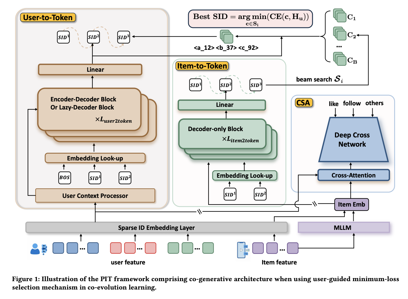
PIT consists of three tightly integrated modules:

1. Collaborative Signal Adapter (CSA): A DIN + DCN model that adjusts item multi-modal embeddings by fusing in collaborative signals. The data is organized in a pointwise format — each item’s multi-modal embedding is refined through interaction with collaborative filtering features, producing a representation that blends content understanding with behavioral patterns.

2. Item-to-Token Module: A decoder-only Transformer (0.1B parameters) that takes the CSA-refined embedding as the BOS token embedding and autoregressively decodes it into a sequence of SID tokens. Both the Item-to-Token and User-to-Token modules share a vocabulary size of $8192 \times 3$.

3. User-to-Token Module: An encoder-decoder architecture that takes the user’s behavior sequence as input (processed by the encoder) and decodes SID tokens for the next-item prediction. The DIN model uses a simplified architecture consisting of a 4-layer MLP and a single cross-attention Transformer layer.

Training: Warm-up and RL-Inspired Co-Training

Training proceeds in two phases:

Phase 1 — Warm-up: All three components are trained simultaneously using pre-generated SIDs as supervision. This bootstraps the system and establishes initial alignment between the item tokenizer and the recommendation model.

Phase 2 — Joint Co-Training: This phase introduces an RL-inspired training loop:

1. The Item-to-Token module performs beam search to generate multiple SID candidates for each item.
2. Among all candidates, the one that minimizes the User-to-Token module’s NTP loss is selected as the target.
3. All three modules are then updated using this selected SID as the training signal.

This mechanism is conceptually similar to rejection sampling in RL — the Item-to-Token module proposes candidates, and the User-to-Token module acts as a critic that selects the best one. Over training iterations, the Item-to-Token module learns to generate SIDs that are not only semantically meaningful but also maximally useful for the downstream recommendation task.

Dynamic SID-Item Index

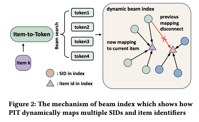
A key practical contribution is the graph-based SID-item index. Rather than maintaining a static mapping table, PIT organizes the SID-item relationships as a weighted graph, where edge weights are updated dynamically as the model evolves. This design is likely motivated by Kuaishou’s existing graph engine infrastructure for online serving, enabling seamless integration with their production systems.

This graph-based approach addresses a fundamental limitation of traditional SID systems: when the model is retrained or fine-tuned, the SID assignments may shift, requiring a full rebuild of the mapping index. PIT’s weighted graph naturally accommodates gradual changes through weight updates rather than wholesale reconstruction.

Key Takeaways

1. Long-sequence compression is converging on learnable memory tokens. Both Tencent’s Recurrent Preference Memory and Meta’s earlier work adopt the same fundamental approach — segmenting user sequences and compressing each segment through a learnable token. The innovation frontier has shifted to how these tokens are trained: Tencent’s self-reflection teacher forcing offers a compelling balance between training parallelism and memory fidelity.

2. Constrained decoding performance is a deployment bottleneck worth solving. Google’s trie vectorization work highlights that even with a well-trained generative model, the constrained beam search step can be a significant serving bottleneck. The hybrid dense/CSR representation, combined with static shape guarantees for accelerator compilers, is a practical and elegant solution that enables branchless execution on TPUs and GPUs.

3. Static SID pipelines are being challenged. PIT’s co-training approach fundamentally rethinks the SID lifecycle. Rather than treating SID generation as a preprocessing step disconnected from the recommendation model, PIT trains them jointly — allowing the SIDs to evolve with the model. Combined with the graph-based dynamic index, this represents a meaningful step toward production-friendly SID systems that can adapt without full pipeline rebuilds.

If you find this post helpful, feel free to scan the QR code below to support me and treat me to a cup of coffee